import pandas as pd
import numpy as np
import matplotlib.pyplot as plt
import seaborn as snsTutorial 4 - Seaborn e GeoPandas
Aprendendo a fazer gráficos mais avançados
Carregando os pacotes
Lendo os dados
Você pode baixar os dados aqui.
imdb_filmes = pd.read_csv("pydata3/imdb_filmes.csv")imdb_filmes.info()<class 'pandas.core.frame.DataFrame'>
RangeIndex: 11340 entries, 0 to 11339
Data columns (total 20 columns):
# Column Non-Null Count Dtype
--- ------ -------------- -----
0 id_filme 11340 non-null object
1 titulo 11340 non-null object
2 ano 11339 non-null float64
3 data_lancamento 11340 non-null object
4 generos 11340 non-null object
5 duracao 11340 non-null int64
6 pais 11340 non-null object
7 idioma 11261 non-null object
8 orcamento 6389 non-null float64
9 receita 6366 non-null float64
10 receita_eua 5997 non-null float64
11 nota_imdb 11340 non-null float64
12 num_avaliacoes 11340 non-null int64
13 direcao 11340 non-null object
14 roteiro 11325 non-null object
15 producao 11220 non-null object
16 elenco 11336 non-null object
17 descricao 11326 non-null object
18 num_criticas_publico 11330 non-null float64
19 num_criticas_critica 11300 non-null float64
dtypes: float64(7), int64(2), object(11)
memory usage: 1.7+ MBimdb_filmes.describe()| ano | duracao | orcamento | receita | receita_eua | nota_imdb | num_avaliacoes | num_criticas_publico | num_criticas_critica | |
|---|---|---|---|---|---|---|---|---|---|
| count | 11339.000000 | 11340.000000 | 6.389000e+03 | 6.366000e+03 | 5.997000e+03 | 11340.000000 | 1.134000e+04 | 11330.000000 | 11300.000000 |
| mean | 1989.452244 | 99.691975 | 1.903052e+07 | 5.468264e+07 | 3.147534e+07 | 6.102487 | 3.591951e+04 | 138.221977 | 65.660885 |
| std | 25.548495 | 17.649559 | 3.238295e+07 | 1.433980e+08 | 6.033264e+07 | 1.128953 | 1.051027e+05 | 303.109281 | 85.890610 |
| min | 1914.000000 | 45.000000 | 0.000000e+00 | 1.600000e+01 | 2.520000e+02 | 1.300000 | 1.001000e+03 | 1.000000 | 1.000000 |
| 25% | 1973.000000 | 89.000000 | 1.500000e+06 | 5.030680e+05 | 1.007583e+06 | 5.500000 | 1.877000e+03 | 31.000000 | 17.000000 |
| 50% | 1997.000000 | 97.000000 | 6.500000e+06 | 9.521381e+06 | 1.067257e+07 | 6.300000 | 4.736500e+03 | 55.000000 | 35.000000 |
| 75% | 2011.000000 | 108.000000 | 2.200000e+07 | 4.309351e+07 | 3.600150e+07 | 6.900000 | 2.106250e+04 | 127.000000 | 78.000000 |
| max | 2020.000000 | 271.000000 | 3.560000e+08 | 2.797801e+09 | 9.366622e+08 | 9.300000 | 2.278845e+06 | 8869.000000 | 909.000000 |
imdb_filmes.sample(8)| id_filme | titulo | ano | data_lancamento | generos | duracao | pais | idioma | orcamento | receita | receita_eua | nota_imdb | num_avaliacoes | direcao | roteiro | producao | elenco | descricao | num_criticas_publico | num_criticas_critica | |
|---|---|---|---|---|---|---|---|---|---|---|---|---|---|---|---|---|---|---|---|---|
| 9250 | tt0119223 | Great Expectations | 1998.0 | 1998-03-02 | Drama, Romance | 111 | USA | English, French, Portuguese | 25000000.0 | 55494066.0 | 26420672.0 | 6.9 | 50455 | Alfonso Cuarón | Charles Dickens, Mitch Glazer | Art Linson Productions | Ethan Hawke, Gwyneth Paltrow, Hank Azaria, Chr... | Modernization of Charles Dickens classic story... | 208.0 | 81.0 |
| 6397 | tt0145529 | Time Chasers | 1994.0 | 1994-03-17 | Sci-Fi | 89 | USA | English | 150000.0 | NaN | NaN | 2.4 | 3041 | David Giancola | David Giancola | Edgewood Studios | Matthew Bruch, Bonnie Pritchard, Peter Harring... | An inventor comes up with a time machine, but ... | 89.0 | 7.0 |
| 7101 | tt0058371 | The Moon-Spinners | 1964.0 | 1964-07-08 | Adventure, Family, Mystery | 118 | USA | English, Greek, Spanish | 5000000.0 | NaN | NaN | 6.7 | 2137 | James Neilson | Michael Dyne, Mary Stewart | Walt Disney Productions | Hayley Mills, Eli Wallach, Peter McEnery, Joan... | A teenager encounters romance, intrigue and a ... | 42.0 | 10.0 |
| 10576 | tt0198781 | Monsters, Inc. | 2001.0 | 2002-03-15 | Animation, Adventure, Comedy | 92 | USA | English | 115000000.0 | 578981070.0 | 289916256.0 | 8.0 | 794964 | Pete Docter, David Silverman | Pete Docter, Jill Culton | Pixar Animation Studios | John Goodman, Billy Crystal, Mary Gibbs, Steve... | In order to power the city, monsters have to s... | 687.0 | 264.0 |
| 10292 | tt1713476 | The Bay | 2012.0 | 2013-06-06 | Horror, Sci-Fi, Thriller | 84 | USA | English | NaN | 1581252.0 | 30668.0 | 5.6 | 24893 | Barry Levinson | Michael Wallach, Barry Levinson | Automatik Entertainment | Nansi Aluka, Christopher Denham, Stephen Kunke... | Chaos breaks out in a small Maryland town afte... | 152.0 | 223.0 |
| 1260 | tt3203620 | The Dinner | 2017.0 | 2017-05-18 | Crime, Drama, Thriller | 120 | USA | English | NaN | 2544921.0 | 1323312.0 | 4.5 | 7518 | Oren Moverman | Herman Koch, Oren Moverman | ChubbCo Film | Michael Chernus, Taylor Rae Almonte, Steve Coo... | Two sets of wealthy parents meet for dinner to... | 193.0 | 120.0 |
| 1126 | tt0087795 | Night Patrol | 1984.0 | 1984-11-16 | Comedy | 85 | USA | French, English | 4500000.0 | NaN | NaN | 4.9 | 1314 | Jackie Kong | Murray Langston, William A. Levey | RSL | Linda Blair, Pat Paulsen, Jaye P. Morgan, Jack... | A hapless police officer is transferred to the... | 34.0 | 16.0 |
| 117 | tt0064683 | Mondo Trasho | 1969.0 | 1969-03-14 | Comedy | 95 | USA | English | 2100.0 | NaN | NaN | 6.2 | 1169 | John Waters | John Waters | Dreamland | Mary Vivian Pearce, Divine, David Lochary, Min... | A day in the lives of a hit-and-run driver and... | 22.0 | 18.0 |
Limpeza dos dados
Vamos converter a coluna data_lancamento para formato data.
# Get all unique non-date values from `data_lancamento`
non_date_values = imdb_filmes[pd.to_datetime(imdb_filmes['data_lancamento'], errors='coerce').isna()]['data_lancamento'].unique()

if (len(non_date_values) > 20):
  # Sample 20 of them if there are too many unique values
  print(f"Non-date values in `data_lancamento`: {np.random.choice(non_date_values, 20, replace=False)}")
else:
  # Otherwise print all unique non-date values from `data_lancamento`
  print(f"Non-date values in `data_lancamento`: {non_date_values}")
Non-date values in `data_lancamento`: ['1934' '1988' '1922' '1996' '1950' '1974' '1972' '1977' '1978' '1936'
'1998' '2018' '1959' '1997' '1966' '1938' '1954' '2006' '2011' '1951']imdb_filmes['data_lancamento']=pd.to_datetime(imdb_filmes['data_lancamento'], format='%Y-%m-%d',
errors='coerce')Tipos de visualizações
A visualização de dados é uma ferramenta poderosa que não só simplifica a compreensão de grandes volumes de dados, mas também desempenha um papel crucial na estatística aplicada e no aprendizado de máquina. Imagine o potencial de desbloquear insights valiosos e identificar padrões ocultos em seus conjuntos de dados! Com um conhecimento prévio do assunto, você pode explorar as nuances dos dados e revelar conexões significativas que podem surpreender e iluminar tanto você quanto sua audiência.
Gráfico de Dispersão
Quando há necessidade de encontrar correlações, são utilizados os gráficos de dispersão. Se existir um conjunto de dados XY, então um gráfico de dispersão é utilizado para encontrar a relação entre as variáveis X e Y.
As coordenadas x e y devem ser numéricas necessariamente. Vamos usar como exemplo, o dataframe imdb_filmes.
No exemplo, a posição do ponto no eixo x pode ser dada pela coluna orcamento e a posição do ponto no eixo y pela coluna receita.
sns.scatterplot(data=imdb_filmes, x='orcamento', y='receita')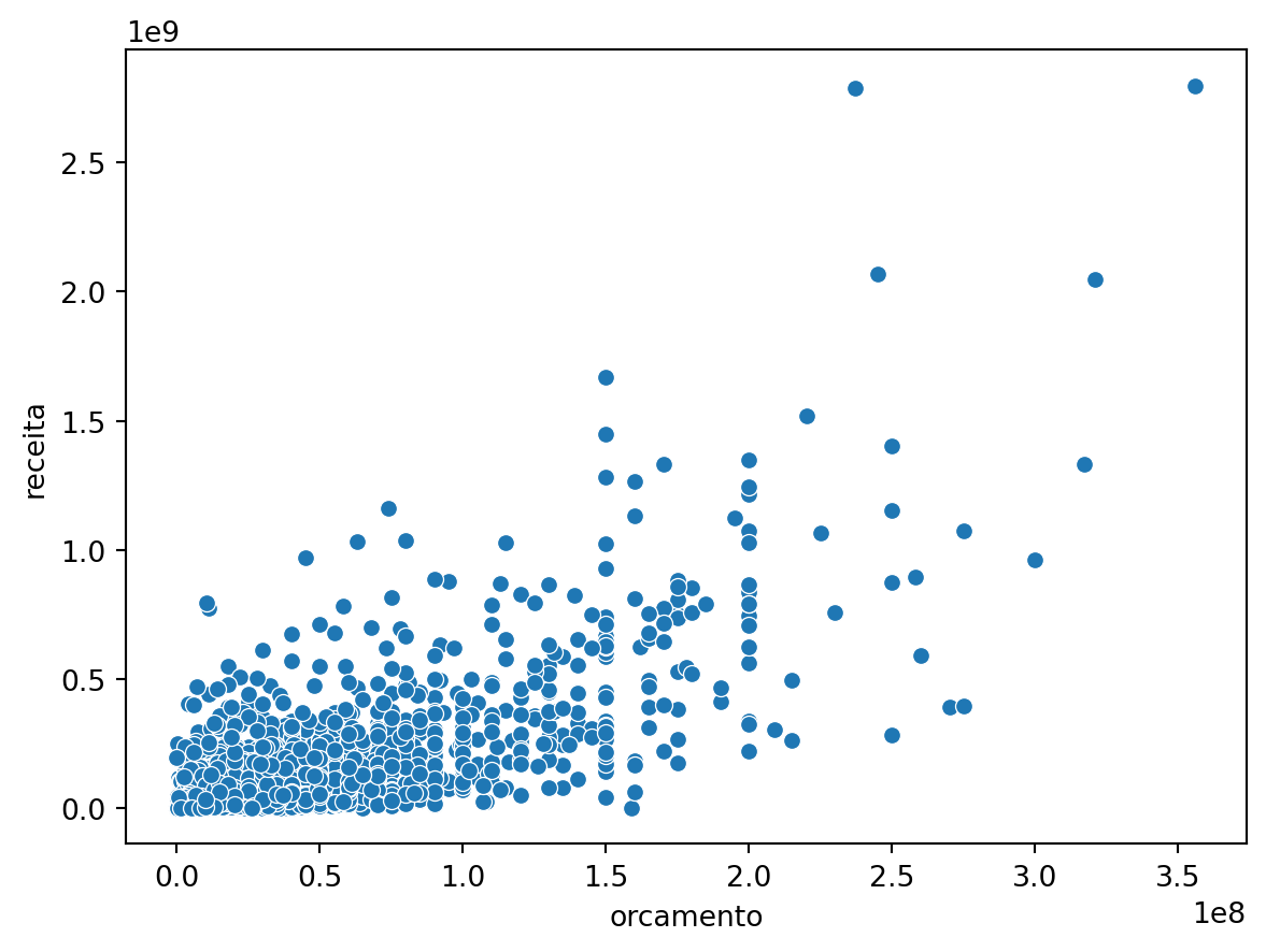
Deixando o gráfico mais informativo:
sns.scatterplot(data=imdb_filmes, x='orcamento', y='receita', hue='ano')

plt.title('Gráfico de Dispersão entre Orçamento x Receita')
plt.xlabel('Orçamento (x 100 Mi UDS)')
plt.ylabel('Receita (Bi USD)')
plt.show()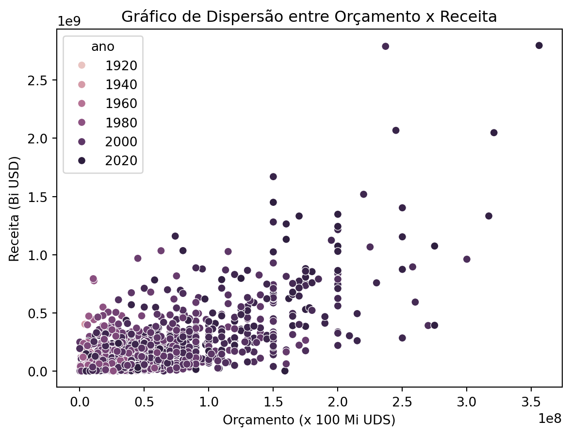
Gráfico de Barras
Um gráfico de barras também exibe tendências ao longo do tempo. No caso de múltiplas variáveis, um gráfico de barras pode facilitar a comparação dos dados para cada variável em todos os momentos no tempo. Por exemplo, um gráfico de barras pode ser utilizado para comparar o crescimento da empresa ano a ano.
Vamos usar o dataframe imdb_filmes para exemplificar, ordenando as linhas por ordem decrescente de nota_imdb. Primeiro vamos gerar o gráfico com as configuração padrão.
imdb_summary = imdb_filmes.sort_values('nota_imdb',
ascending=False).head(8)
sns.barplot(imdb_summary, x='titulo', y='nota_imdb')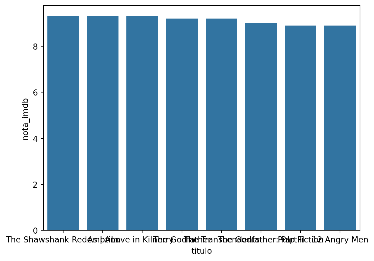
Mas os nomes dos filmes estão sobrepostos, então neste caso é recomendável realizar um gráfico de barras horizontais.
sns.barplot(imdb_summary, x='nota_imdb', y='titulo')
plt.title('Top 10 Filmes por Nota IMDB')
plt.xlabel('Nota IMDB')
plt.show()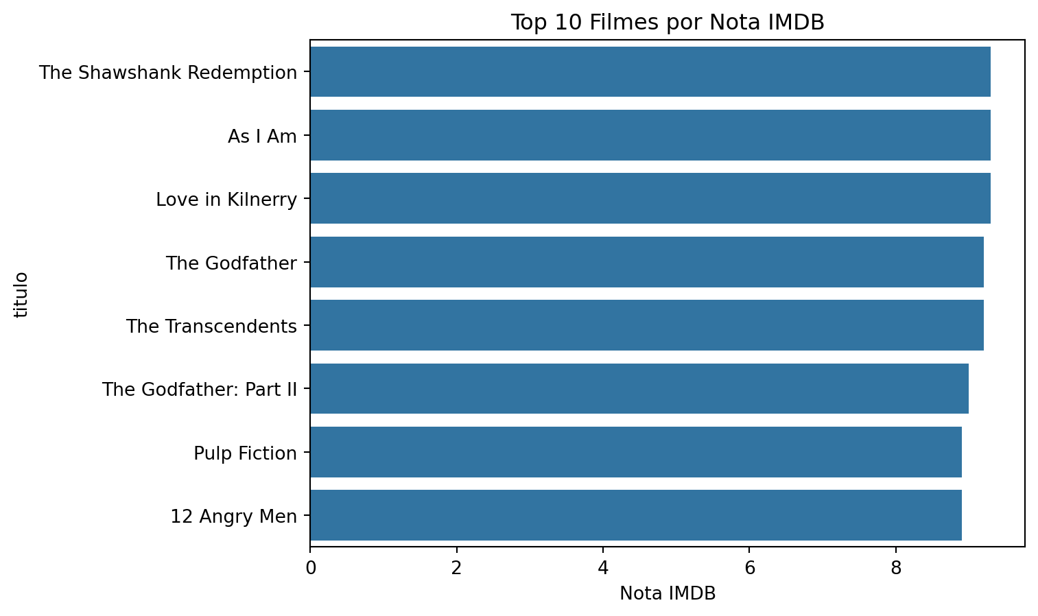
Gráfico de linha
Gráficos de linhas são utilizados para exibir tendências ao longo do tempo. O eixo X é geralmente utilizado para representar um período, enquanto o eixo Y é utilizado para representar a quantidade associada ao período de tempo no eixo X. Por exemplo, um gráfico de linhas pode ilustrar o horário de pico de visitas em um shopping durante o dia, dividido por dias da semana e horas.
Vamos fazer um gráfico utilizando a coluna data_lancamento
imdb_lancamento = imdb_filmes.groupby('data_lancamento').agg({'titulo':"count",'nota_imdb':'mean','duracao':'mean'})

imdb_lancamento.head(3)| titulo | nota_imdb | duracao | |
|---|---|---|---|
| data_lancamento | |||
| 1914-03-08 | 1 | 6.1 | 61.0 |
| 1914-08-24 | 1 | 6.4 | 78.0 |
| 1914-12-21 | 1 | 6.3 | 82.0 |
Vamos agrupar os filmes por ano.
imdb_anual = imdb_filmes.groupby(pd.Grouper(key='data_lancamento', freq='Y'))['nota_imdb'].mean()

imdb_anual.head(3)
data_lancamento
1914-12-31 6.266667
1915-12-31 6.566667
1916-12-31 6.200000
Name: nota_imdb, dtype: float64imdb_anual_df = pd.DataFrame(imdb_anual).reset_index()
imdb_anual_df['data_lancamento'] = pd.to_datetime(imdb_anual_df['data_lancamento'], format='%Y-%m-%d')
sns.lineplot(x='data_lancamento', y='nota_imdb', data=imdb_anual_df)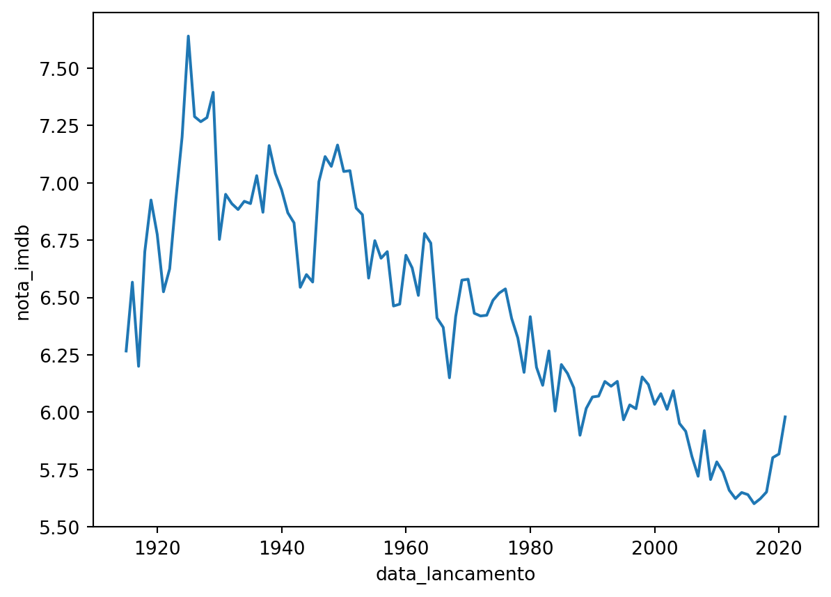
Também podemos plotar duas ou mais linhas. Vamos calcular intervalo interquartil e inclui-la no gráfico anterior.
Gráfico de Boxplot
Um gráfico de boxplot, também conhecido como diagrama de caixa, é uma ferramenta de visualização estatística que fornece uma representação compacta e informativa da distribuição de um conjunto de dados. Consiste em um retângulo (“caixa”) que se estende de um quartil ao outro, com uma linha vertical (ou “whisker”) estendendo-se de cada extremidade da caixa para representar a amplitude dos dados fora do intervalo interquartil.
imdb_filmes['ano'] = imdb_filmes['data_lancamento'].dt.year

imdb_filmes['decada'] = imdb_filmes['ano'] // 10 * 10

imdb_filmes['decada'].astype('category')
0 1980.0
1 1940.0
2 2000.0
3 1940.0
4 2000.0
...
11335 NaN
11336 2010.0
11337 1950.0
11338 2010.0
11339 2000.0
Name: decada, Length: 11340, dtype: category
Categories (12, float64): [1910.0, 1920.0, 1930.0, 1940.0, ..., 1990.0, 2000.0, 2010.0, 2020.0]sns.boxplot(x='decada', y='nota_imdb', data=imdb_filmes, showmeans=True)
plt.title('Distribuição de notas IMDB por Década')
plt.ylabel('IMDb Rating')
plt.show()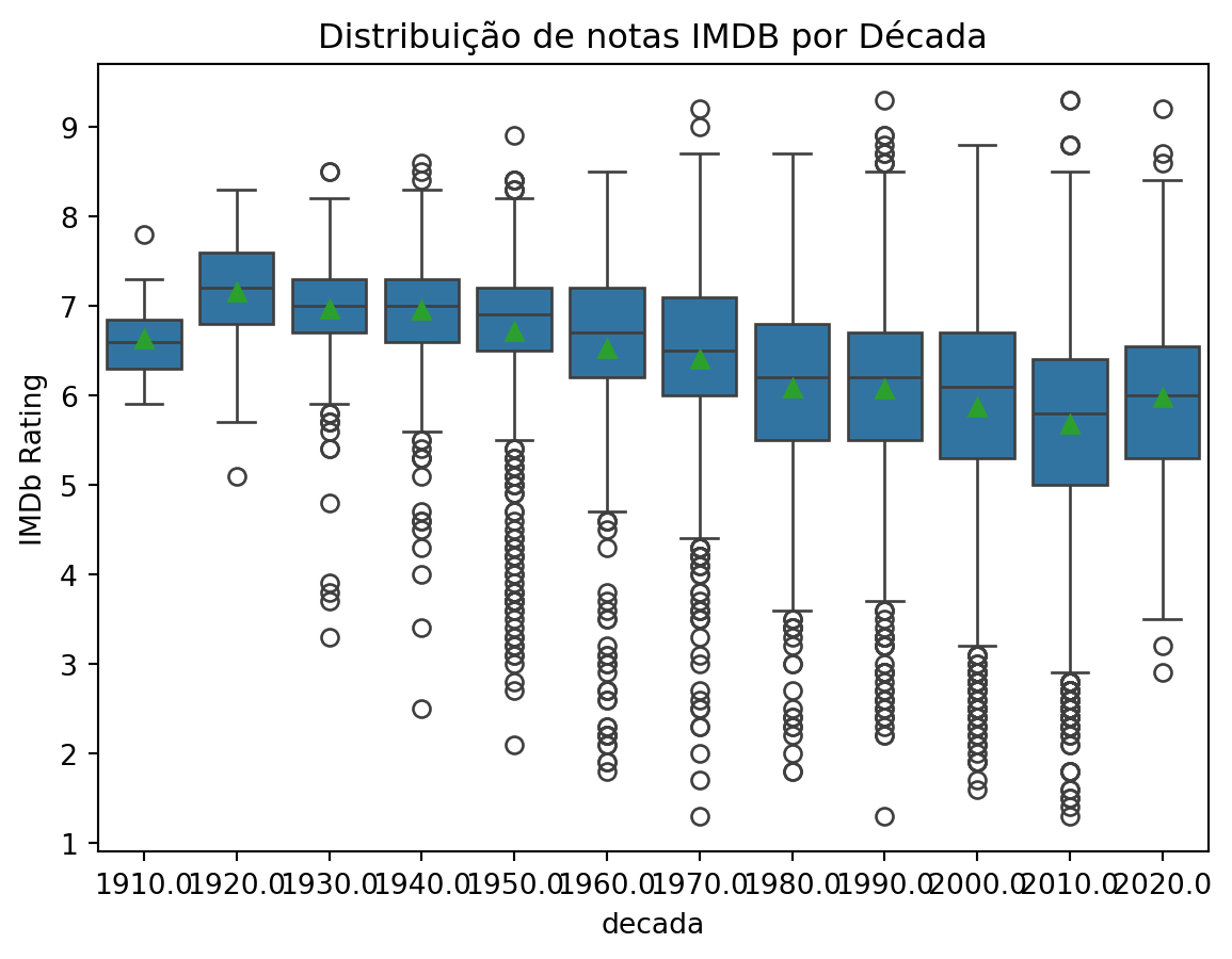
O gráfico ficou ruim de visualizar, porém, é possível alterar as dimensões de qualquer gráfico matplotlib, utilizando a opção: plt.figure(figsize=(15, 8)). Também podemos mudar a cor de cada caixa.
plt.figure(figsize=(15, 8))
sns.boxplot(x='decada', y='nota_imdb', hue='decada', data=imdb_filmes, showmeans=True)
plt.title('Distribuição de notas IMDB por Década')
plt.ylabel('IMDb Rating')
plt.show()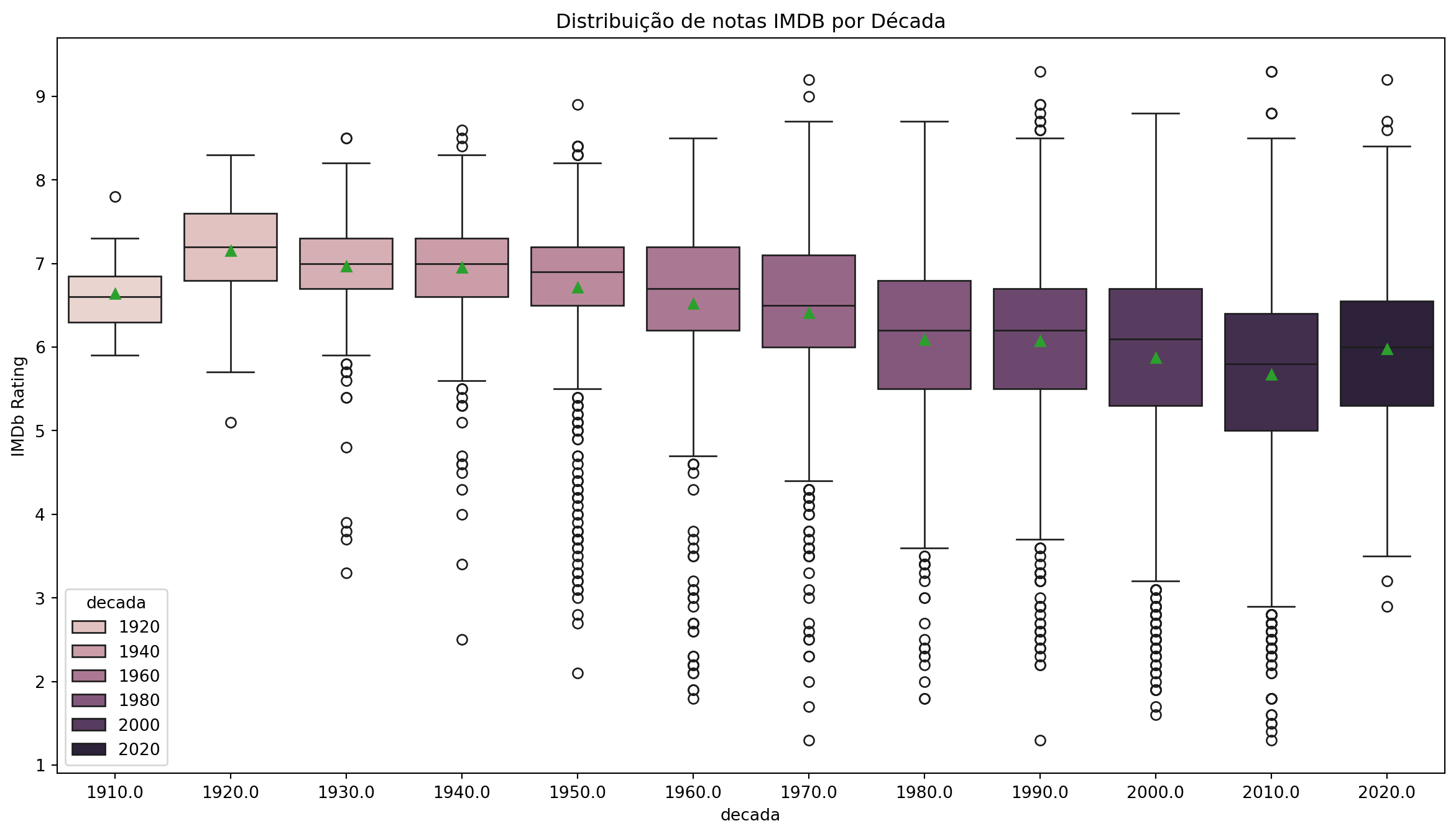
Gráfico de Histograma
Um histograma representa dados usando barras de alturas diferentes. Geralmente, cada barra agrupa números em intervalos em um histograma. Quanto mais alta as barras, mais dados se encaixam nesse intervalo. É usado para exibir a forma e a dispersão de amostras de um conjunto de dados contínuos. Por exemplo, podemos usar um histograma para medir as frequências de resposta da variável nota_imdb .
O Histograma serve para observar a distribuição dos dados e eventualmente serve para comparar mais de uma distribuição.
sns.histplot(data=imdb_filmes, x='nota_imdb',
bins=30, color='darkblue')
plt.xlabel('Nota IMDb')
plt.show()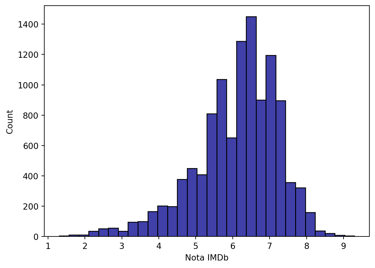
Mapas
Precisamos instalar alguns pacotes:
pip install geobrpip install geopandas
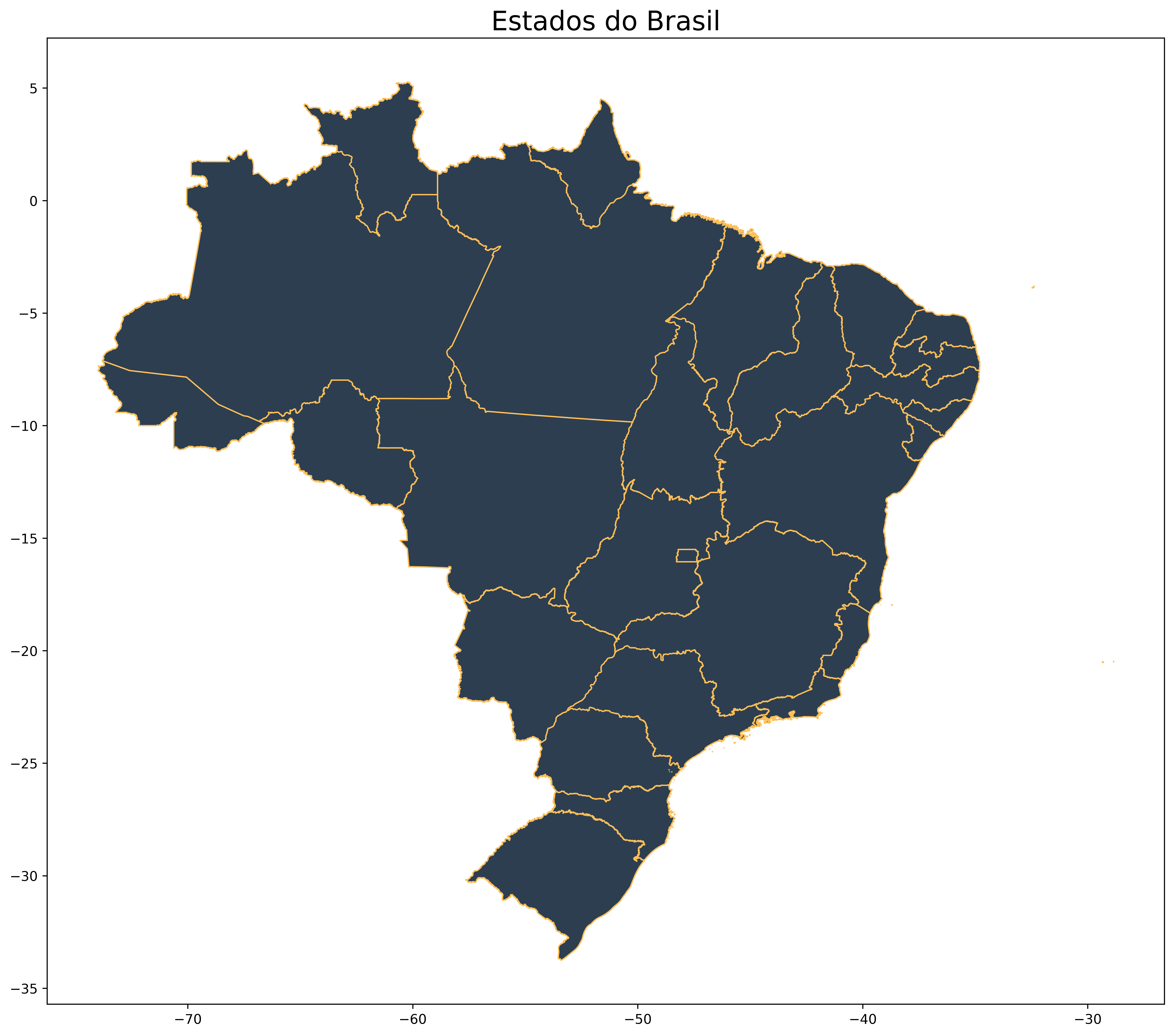
Pacote geobr para mapas do Brasil
Vamos baixar os dados do Brasil por Estados.
import numpy as np
import geobr
import geopandas as gpd

states = geobr.read_state(year=2019)
/Users/mauricio/Library/Python/3.8/lib/python/site-packages/urllib3/__init__.py:35: NotOpenSSLWarning:
urllib3 v2 only supports OpenSSL 1.1.1+, currently the 'ssl' module is compiled with 'LibreSSL 2.8.3'. See: https://github.com/urllib3/urllib3/issues/3020
/Users/mauricio/Library/Python/3.8/lib/python/site-packages/geopandas/array.py:93: ShapelyDeprecationWarning:
__len__ for multi-part geometries is deprecated and will be removed in Shapely 2.0. Check the length of the `geoms` property instead to get the number of parts of a multi-part geometry.
fig, ax = plt.subplots(figsize=(15, 15), dpi=300)
states.plot(facecolor="#2D3E50", edgecolor="#FEBF57", ax=ax)
ax.set_title("Estados do Brasil", fontsize=20)
plt.show()
/Users/mauricio/Library/Python/3.8/lib/python/site-packages/geopandas/plotting.py:33: ShapelyDeprecationWarning:
Iteration over multi-part geometries is deprecated and will be removed in Shapely 2.0. Use the `geoms` property to access the constituent parts of a multi-part geometry.
/Users/mauricio/Library/Python/3.8/lib/python/site-packages/descartes/patch.py:62: ShapelyDeprecationWarning:
The array interface is deprecated and will no longer work in Shapely 2.0. Convert the '.coords' to a numpy array instead.
/Users/mauricio/Library/Python/3.8/lib/python/site-packages/descartes/patch.py:64: ShapelyDeprecationWarning:
The array interface is deprecated and will no longer work in Shapely 2.0. Convert the '.coords' to a numpy array instead.
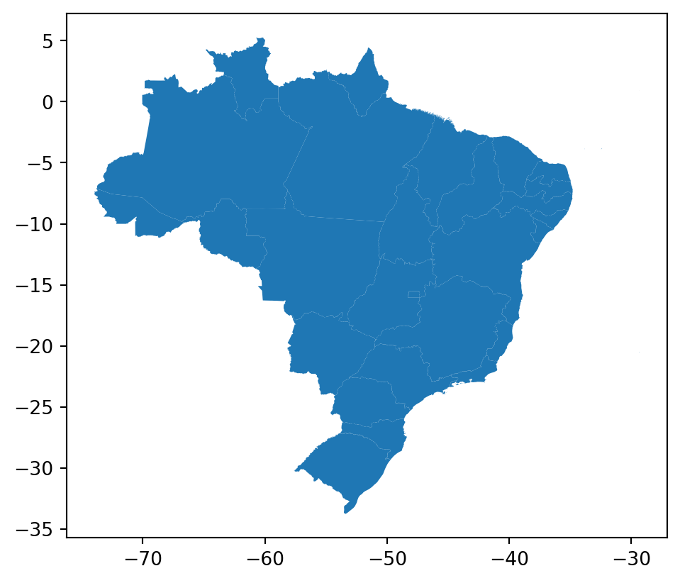
Outra forma de trabalhar manualmente o mapa é utilizando a library geopandas e importando diretamente os dados geográficos.
Você pode baixar os dados aqui.
Vamos baixar os dados do Brasil do seguinte endereço:
www.ibge.gov.br –> geociências –> downloads –> cartas e mapas –> bases cartográficas contínuas –> bcim –> versao 2016 –> geopackage
mapa = gpd.read_file('pydata4/bcim_2016_21_11_2018.gpkg', layer='lim_unidade_federacao_a')/Users/mauricio/Library/Python/3.8/lib/python/site-packages/geopandas/array.py:93: ShapelyDeprecationWarning:
__len__ for multi-part geometries is deprecated and will be removed in Shapely 2.0. Check the length of the `geoms` property instead to get the number of parts of a multi-part geometry.
mapa.head()| nome | nomeabrev | geometriaaproximada | sigla | geocodigo | id_produtor | id_elementoprodutor | cd_insumo_orgao | nr_insumo_mes | nr_insumo_ano | tx_insumo_documento | geometry | |
|---|---|---|---|---|---|---|---|---|---|---|---|---|
| 0 | Goiás | None | Sim | GO | 52 | 1000001 | None | NaN | None | None | None | MULTIPOLYGON (((-50.15876 -12.41581, -50.15743... |
| 1 | Mato Grosso do Sul | None | Sim | MS | 50 | 1000001 | None | NaN | None | None | None | MULTIPOLYGON (((-56.09815 -17.17220, -56.09159... |
| 2 | Paraná | None | Sim | PR | 41 | 1000001 | None | NaN | None | None | None | MULTIPOLYGON (((-52.08090 -22.52893, -52.04903... |
| 3 | Minas Gerais | None | Sim | MG | 31 | 1000001 | None | NaN | None | None | None | MULTIPOLYGON (((-44.21152 -14.22955, -44.20750... |
| 4 | Sergipe | None | Sim | SE | 28 | 1000001 | None | NaN | None | None | None | MULTIPOLYGON (((-38.00366 -9.51544, -38.00052 ... |
Vamos a plotar o mapa do Brasil
mapa.plot()/Users/mauricio/Library/Python/3.8/lib/python/site-packages/geopandas/plotting.py:33: ShapelyDeprecationWarning:
Iteration over multi-part geometries is deprecated and will be removed in Shapely 2.0. Use the `geoms` property to access the constituent parts of a multi-part geometry.
/Users/mauricio/Library/Python/3.8/lib/python/site-packages/descartes/patch.py:62: ShapelyDeprecationWarning:
The array interface is deprecated and will no longer work in Shapely 2.0. Convert the '.coords' to a numpy array instead.
/Users/mauricio/Library/Python/3.8/lib/python/site-packages/descartes/patch.py:64: ShapelyDeprecationWarning:
The array interface is deprecated and will no longer work in Shapely 2.0. Convert the '.coords' to a numpy array instead.
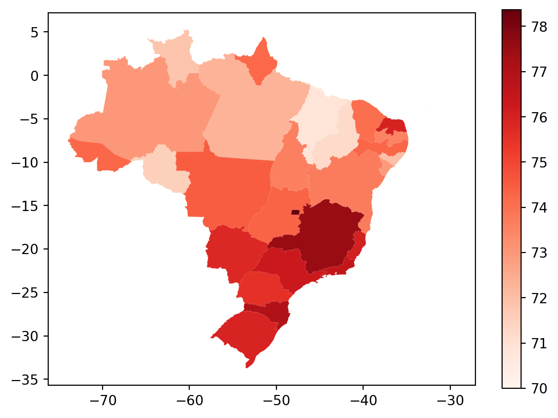
Agora queremos mapear alguma informação. Como exemplo, vamos pegar dados da expectativa de vida para os estados brasileiros:
vida = pd.read_csv('pydata4/br_states_lifexpect2017.csv')
vida.info()
<class 'pandas.core.frame.DataFrame'>
RangeIndex: 27 entries, 0 to 26
Data columns (total 3 columns):
# Column Non-Null Count Dtype
--- ------ -------------- -----
0 X 27 non-null int64
1 uf 27 non-null object
2 ESPVIDA2017 27 non-null float64
dtypes: float64(1), int64(1), object(1)
memory usage: 776.0+ bytesVamos unir as informações dos dois dataframes.
br = pd.merge(mapa, vida, left_on='nome',right_on='uf', how='left')
br= br.fillna(73)
Finalmente, vamos plotar o mapa:
vmax = np.max(br['ESPVIDA2017'])
vmin=np.min(br['ESPVIDA2017'])

br.plot(column='ESPVIDA2017',
        legend=True,
        cmap='Reds',
        vmax=vmax,
        vmin=70)
plt.show()
/Users/mauricio/Library/Python/3.8/lib/python/site-packages/geopandas/plotting.py:33: ShapelyDeprecationWarning:
Iteration over multi-part geometries is deprecated and will be removed in Shapely 2.0. Use the `geoms` property to access the constituent parts of a multi-part geometry.
/Users/mauricio/Library/Python/3.8/lib/python/site-packages/descartes/patch.py:62: ShapelyDeprecationWarning:
The array interface is deprecated and will no longer work in Shapely 2.0. Convert the '.coords' to a numpy array instead.
/Users/mauricio/Library/Python/3.8/lib/python/site-packages/descartes/patch.py:64: ShapelyDeprecationWarning:
The array interface is deprecated and will no longer work in Shapely 2.0. Convert the '.coords' to a numpy array instead.
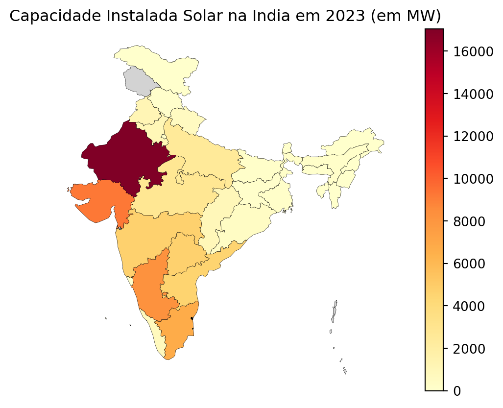
Exemplo com dados de outro pais
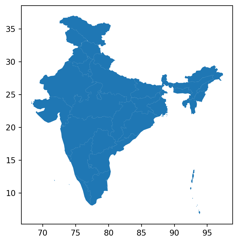
mapa_india = gpd.read_file('pydata4/india/india-polygon.shp')

mapa_india.head(3)
/Users/mauricio/Library/Python/3.8/lib/python/site-packages/geopandas/array.py:93: ShapelyDeprecationWarning:
__len__ for multi-part geometries is deprecated and will be removed in Shapely 2.0. Check the length of the `geoms` property instead to get the number of parts of a multi-part geometry.
| id | st_nm | geometry | |
|---|---|---|---|
| 0 | None | Andaman and Nicobar Islands | MULTIPOLYGON (((93.84831 7.24028, 93.92705 7.0... |
| 1 | None | Arunachal Pradesh | POLYGON ((95.23643 26.68105, 95.19594 27.03612... |
| 2 | None | Assam | POLYGON ((95.19594 27.03612, 95.08795 26.94578... |
mapa_india.plot()/Users/mauricio/Library/Python/3.8/lib/python/site-packages/geopandas/plotting.py:33: ShapelyDeprecationWarning:
Iteration over multi-part geometries is deprecated and will be removed in Shapely 2.0. Use the `geoms` property to access the constituent parts of a multi-part geometry.
/Users/mauricio/Library/Python/3.8/lib/python/site-packages/descartes/patch.py:62: ShapelyDeprecationWarning:
The array interface is deprecated and will no longer work in Shapely 2.0. Convert the '.coords' to a numpy array instead.
/Users/mauricio/Library/Python/3.8/lib/python/site-packages/descartes/patch.py:64: ShapelyDeprecationWarning:
The array interface is deprecated and will no longer work in Shapely 2.0. Convert the '.coords' to a numpy array instead.
Vamos mapear os dados provenientes de:
dados_india = pd.read_excel('pydata4/importIN.xlsx')
dados_india.head(3)

dados_india2023 = dados_india[['Year',2023]]
Juntando os dados
mapa_india_2023 = pd.merge(mapa_india, dados_india2023,
left_on = 'st_nm', right_on='Year', how='left')

mapa_india_2023.head(3)| id | st_nm | geometry | Year | 2023 | |
|---|---|---|---|---|---|
| 0 | None | Andaman and Nicobar Islands | MULTIPOLYGON (((93.84831 7.24028, 93.92705 7.0... | NaN | NaN |
| 1 | None | Arunachal Pradesh | POLYGON ((95.23643 26.68105, 95.19594 27.03612... | Arunachal Pradesh | 11.64 |
| 2 | None | Assam | POLYGON ((95.19594 27.03612, 95.08795 26.94578... | Assam | 147.92 |
Agora vamos plotar:
np.min(mapa_india_2023[2023])3.04np.min(mapa_india_2023[2023])
mapa_india_2023.plot(column=2023,
missing_kwds={'color':'lightgrey'},
legend=True,
cmap='YlOrRd',
linewidth=0.2,
edgecolor='0',
vmin=0).set_axis_off()
plt.title('Capacidade Instalada Solar na India em 2023 (em MW)')
plt.show()/Users/mauricio/Library/Python/3.8/lib/python/site-packages/geopandas/plotting.py:33: ShapelyDeprecationWarning:
Iteration over multi-part geometries is deprecated and will be removed in Shapely 2.0. Use the `geoms` property to access the constituent parts of a multi-part geometry.
/Users/mauricio/Library/Python/3.8/lib/python/site-packages/descartes/patch.py:62: ShapelyDeprecationWarning:
The array interface is deprecated and will no longer work in Shapely 2.0. Convert the '.coords' to a numpy array instead.
/Users/mauricio/Library/Python/3.8/lib/python/site-packages/descartes/patch.py:64: ShapelyDeprecationWarning:
The array interface is deprecated and will no longer work in Shapely 2.0. Convert the '.coords' to a numpy array instead.
/Users/mauricio/Library/Python/3.8/lib/python/site-packages/geopandas/plotting.py:33: ShapelyDeprecationWarning:
Iteration over multi-part geometries is deprecated and will be removed in Shapely 2.0. Use the `geoms` property to access the constituent parts of a multi-part geometry.
/Users/mauricio/Library/Python/3.8/lib/python/site-packages/descartes/patch.py:62: ShapelyDeprecationWarning:
The array interface is deprecated and will no longer work in Shapely 2.0. Convert the '.coords' to a numpy array instead.